DP11: Superintelligence and Statistical Sleuth

Mission #9.
Mail dated Aug 13,
Great job on spending 29 hours in a week! I recommend measuring rate of phrases per hour.
Overall, I didn’t see you take on Superintelligence, which was the mission. Please work on either that or stuff you feel confused about. Only failures matter (apart from maintenance of existing performance).
Note down patterns of failure, such as “X prefers A to B”. Spend, say, half your time searching for and practicing on examples of those types. You can spend the rest of your practice time on new examples, from which you will hopefully find other patterns of failure.
Mail dated June 24,
Mission #9: Your mission, should you choose to accept it, is to concretely analyze the key claims in the book Superintelligence by Nick Bostrom (the book mentioned in the Elon Musk tweet above). He’s a PhD at Oxford who’s been writing about AI safety along with guys like Eliezer for nearly two decades. The book has detailed arguments and examples about all the topics like possible paths to “superintelligence” (whatever that means), types of “superintelligence”, the control problem, etc.
No need to write “Question: “ - doesn’t seem to have changed your answers.
Don’t have to go sentence by sentence; look at one key claim for each section, usually the one in the first few paragraphs, or one for each paragraph if you feel it’s an important section. For example:
CHAPTER 2 Paths to superintelligence
Machines are currently far inferior to humans in general intelligence. Yet one day (we have suggested) they will be superintelligent. How do we get from here to there? This chapter explores several conceivable technological paths. We look at artificial intelligence, whole brain emulation, biological cognition, and human-machine interfaces, as well as networks and organizations. We evaluate their different degrees of plausibility as pathways to superintelligence. The existence of multiple paths increases the probability that the destination can be reached via at least one of them.
The key claim is “How do we get from here to there? Answer: Artificial intelligence, whole brain emulation, …”
Feedback checklist:
-
Could it be that this claim has no any example at all? For example, “civilization is at stake”.
-
Could this claim be false? Remember the “there is no doubting” example.
-
Does this claim say anything about “best” (need to compare against the entire set) or “most” (need to show it’s the majority in the set) or “no” (need to show that nothing in the set matches)?
-
Did you stick to examples that are in the chapter itself? That way you don’t have to search online for too long.
-
Did you use a running example for a technical phrase? There will be lots of new phrases in the book, like “convergent instrumental value” and “orthogonality thesis”. Whenever you see them, you should recall whatever running example you’ve used.
-
If this is an “if-then” claim, did you either get a concrete example or mark it as having no example?
Short names: none; false; best; chapter; running; if-then.
Please refer to the checklist after every claim analysis to ensure you’re not making old mistakes. If you want to add to the checklist based on mistakes found in past feedback, that’s great.
Introduction
With this Essay I take on the first three chapters of “Superintelligence” by Nick Bostrom, and the first three chapters of Statistical Sleuth. I try to pick “important” claims from each section and try to work them out in the typical DP fashion as is being done since the last essay on “subject-predicate”.
Feedback list used in this essay
For this blog post, I use the checklist that looks like the following:
Checklist: yes; neither;; no-example; failed; (no idea how the example would look); Pattern: “random-sampling?”
In this checklist, “yes” refers to if the claim has an example. “Neither” informs that I don’t know if the claim is true or false based on the example given. The claim has “no-example”, and I have “failed” in it, as I have “no idea how the example would look”. The pattern I suspect that I need to practice more, are claims related to “random sampling”, but I am unsure (?).
I have skipped things like “in-chapter” and “running” as part of my checklists, as I think for most part I have tried to use “running” and “in-chapter” examples. For example, in every chapter of Statistical Sleuth there are two case studies at the beginning of the chapter. I try to use these as much as possible as examples for claims. Where they don’t work, either I have not given examples or I have given other examples in the book, or my own examples.
Regarding “if”, “most/best” etc… I have identified it as a pattern when I have failed in it.
Chapter 1 History
Growth modes and big history
(History at the largest scale)[1], seems to exhibit (a sequence of distinct growth modes)[2], each much more rapid than (its predecessor)[3].
Claims: [1] seems to exhibit [2], each much more rapid than [3].
Subject: [2] exhibited in [1].
Predicate: much more rapid than [3].
Example: “A few hundred thousand years ago, in early human (or hominid) prehistory, growth was so slow that it took in the order of one million years for human productive capacity to increase sufficiently to sustain an additional one million individuals living at subsistence level. By 5000 BC, following the Agricultural Revolution, the rate of growth had increased to the point where the same amount of growth took just two centuries. Today, following the Industrial Revolution, the world economy grows on average by that amount every ninety minutes.”
Definition: checks out.
Checklist: yes; true;
Great expectations
(Machines matching humans in general intelligence)[1]—that is, possessing common sense and an effective ability to learn, reason, and plan to meet complex information-processing challenges across a wide range of natural and abstract domains—have been expected since (the invention of computers in the 1940s)[2].
Claims: [1] has been expected since [2].
Subject: When [1] has been expected since.
Predicate: since [2].
Example: No example of someone expecting in 1940, in the book.
Definition: -
Checklist: yes; neither; no-example;
From the (fact that some individuals have overpredicted artificial intelligence in the past)[1], however, it does not follow that (AI is impossible or will never be developed)[2].
Claims: AI is not impossible or could be developed in the future
Checklist: no; neither; future-with-no-ex;
Claims: From [1], [2] does not follow.
Subject: The future as a result of [1].
Predicate: [2] wont happen.
Example: no-example; Don’t think it is possible to give example for “A leads to or does not lead to B”, atleast in this case.
Definition: -
Checklist: no; neither;;;; if no-example; failed; Pattern: A-leads-to-B; failed (didn’t know if it was possible to give example for this)
The main reason (why progress has been slower than expected)[1] is that (the technical difficulties of constructing intelligent machines have proved greater than the pioneers foresaw)[2].
because
Checklist: yes; neither;
because-should-due-to; time; (I was unsure for a bit if it really
was “because” statement);
Summary of chapter 1
“The AI pioneers for the most part did not countenance the possibility that their enterprise might involve risk. They gave no lip service—let alone serious thought—to any safety concern or ethical qualm related to the creation of artificial minds and potential computer overlords: a lacuna that astonishes even against the background of the era’s not-so-impressive standards of critical technology assessment.”
Seasons of hope and despair
In the (six decades since this brash beginning)[0], (the field of artificial intelligence)[1] has been through (periods of hype and high expectations alternating with periods of setback and disappointment)[2].
Claims: Since [0], [1] has been through [2].
Subject: [1], since [0].
Predicate: has been through [2].
Example: After the Dartmouth meeting, researchers built systems like the Logic Theorist, which was able to prove most of the theorems in the second chapter of WhiteHead and Russell’s Principia Mathematica, and even came up with one proof that was much more elegant than the original.
Post 1970, funding decreased and skepticism increased.
This seems to be the best one can do while giving examples. There are claims in the example (“post 1970…”), but atleast we can ask the author what exactly he meant when needed to investigate further.
Definition: checks out!
Checklist: yes; true;
(The methods)[1] that produced (successes in the early demonstration systems)[2] often proved difficult to (extend to a wider variety of problems or to harder problem instances)[3].
Claims: [1] that produced [2], often proved [3].
Subject: Extension to harder problems based on [2],
Predicate: often proved to be difficult
Example: “For instance, to prove a theorem that has a 5-line long proof in a deduction system with one inference rule and 5 axioms, one could simply enumerate the 3,125 possible combinations and check each one to see if it delivers the intended conclusion”, based on the exhaustive search method.
“Proving a theorem with a 50-line proof does not take ten times longer
than proving a theorem that has a 5-line proof: rather, if one uses
exhaustive search, it requires combing through 5^50 ≈ 8.9 × 10^34
possible sequences—which is computationally infeasible even with the
fastest supercomputers.”
Definition: checks out!
Checklist: yes; true; often; failed; (don’t know how to give an example for often)
State of the art
(Artificial intelligence)[1] already (outperforms human intelligence in many domains)[2].
Claims: [1] already does [2].
Subject: [1].
Predicate: already does [2].
Example: “2010: IBM’s Watson defeats the two all-time-greatest human Jeopardy! champions, Ken Jennings and Brad Rutter. Jeopardy! is a televised game show with trivia questions about history, literature, sports, geography, pop culture, science, and other topics. Questions are presented in the form of clues, and often involve wordplay.” — Games
There are not other examples of [1] already doing [2], in the section.
Definition: Checks out for one domain (gaming) atleast!
Checklist: yes; true;
These achievements might not seem impressive today. But this is because (our standards for what is impressive)[1] keep adapting to the (advances being made)[2].
Claims: [1] keep adapting to the [2].
Subject: [1]
Predicate: keep adapting to [2].
Example: In late fifties: “if one could devise a successful chess machine one would seem to have penetrated to the core of human intellectual endeavor.”
I don’t know anyone who is amazed by a chess AI today. It’s the norm, there are so many apps based on it.
Definition: checks out!
Checklist: yes; true
Opinions about the future of machine intelligence x
Progress on two major fronts—towards a more solid statistical and (information-theoretic foundation for machine learning on the one hand)[1], and (towards the practical and commercial success of various problem-specific or domain-specific applications on the other)[2]—has restored to AI research (some of its lost prestige)[3].
Claims: Progress on [1], and [2], has restored [3] to AI research.
Subject: Progress on [1] and [2].
Predicate: has restored [3] to AI research.
Example: No examples in the section
Definition: -
Checklist: yes; neither; no-example
One result of (this conservatism)[1] has been (increased concentration on “weak AI”—the variety devoted to providing aids to human thought—and away from “strong AI”—the variety that attempts to mechanize human-level intelligence)[2].
Claims: Result of [1] has been [2].
Subject: Result of [1].
Predicate: has been [2].
Example: no examples in the section
Definition: -
Checklist: yes; neither; no-example
(Expert opinions about the future of AI)[1] vary (wildly)[2].
Claims: [1] varies [2].
Subject: [1].
Predicate: varies [2].
Example: A survey documented here shows the prediction of Human-level AI of “experts”, ranging from 2020 all the way to 2100.
Definition: checks out.
Checklist: yes; true;
Summary
“Small sample sizes, selection biases, and—above all—the inherent unreliability of the subjective opinions elicited mean that one should not read too much into these expert surveys and interviews. They do not let us draw any strong conclusion. But they do hint at a weak conclusion. They suggest that (at least in lieu of better data or analysis) it may be reasonable to believe that human-level machine intelligence has a fairly sizeable chance of being developed by mid-century, and that it has a non-trivial chance of being developed considerably sooner or much later;”
Chapter 2 Paths to Superintelligence
Artificial intelligence (8)
How do we get from here to there? AI is a conceivable technology path.
Claims: AI is a conceivable technology path to go from current to superintelligent.
Subject: AI
Predicate: is a conceivable technology path to go from current to superintelligent.
Example: “blind evolutionary processes can produce human-level
general intelligence, since they have already done so at least
once. Evolutionary processes with foresight—that is, genetic programs
designed and guided by an intelligent human programmer—should be able
to achieve a similar outcome with far greater efficiency.”
Crossed out above, are reasons, they are more unverified claims. You can’t give examples for “could be”.
Definition: Also, what does conceivable even mean? How would I know if it is conceivable. How would I know the definition? Maybe if there is an example then it is conceivable?
Checklist: no; neither; future-with-no-ex; definition-unclear;
(Evolutionary processes with foresight—that is, genetic programs)[1] designed and guided by (an intelligent human programmer)[2]—should be able to achieve a (similar outcome with far greater efficiency)[3].
Claims: [1] designed and guided by [2] should be able to achieve [3].
Subject: [1] designed and guided by [2].
Predicate: should be able to achieve [3].
Example:
”If we were to simulate 10^25 neurons over a billion years of
evolution (longer than the existence of nervous systems as we know
them), and we allow our computers to run for one year, these figures
would give us a requirement in the range of 10^31–10^44 FLOPS. For
comparison, China’s Tianhe-2, the world’s most powerful supercomputer
as of September 2013, provides only 3.39×10 16 FLOPS. In recent
decades, it has taken approximately 6.7 years for commodity computers
to increase in power by one order of magnitude. Even a century of
continued Moore’s law would not be enough to close this gap”
This again talks about some prediction for the future. We are not interested in calculations, we are interested for now (for some reason) only in examples
Definition: -
Checklist: no; neither; because-should-due-to; future-with-no-ex
Another way of arguing for the (feasibility of artificial intelligence)[1] is by pointing to the (human brain)[2] and suggesting that we could use it as (a template for a machine intelligence)[3].
Claims: [1] can be done by using [2] as [3].
Subject: [1] using [2] as [3].
Predicate: can be done.
Example: whole brain simulation, taking inspiration from brain,
neuromorphic approaches, recursive self-improvement
Take inspiration all you want. Show me the money (examples)!
Definition: -
Checklist: no; neither; “future with no ex”
Summary
“Lot of ways” to make SI from AI but there are currently 0 examples for it in this section.
Whole brain emulation (6)
Claims: We get from current to superintelligent by using Whole brain Emulation.
Subject: That which will lead us from current to superintelligent
Predicate: is Whole Brain Emulation
Example: “No brain has yet been emulated. Consider the humble
model organism Caenorhabditis elegans, which is a transparent
roundworm, about 1 mm in length, with 302 neurons. The complete
connectivity matrix of these neurons has been known since the
mid-1980s, when it was laboriously mapped out by means of slicing,
electron microscopy, and hand-labeling of specimens…”
There is no example of even a small organism whose brain is emulated currently.
Definition: -
Checklist: no; neither; “future with no ex”
Summary
“Nevertheless, compared with the AI path to machine intelligence, whole brain emulation is more likely to be preceded by clear omens since it relies more on concrete observable technologies and is not wholly based on theoretical insight.”
Biological cognition (8)
Claims: We get from current to superintelligent by using biological cognition.
Subject: That which will lead us from current to superintelligent
Predicate: biological cognition
Example: “Pre-implantation genetic diagnosis has already been
used during in vitro fertilization procedures to screen embryos
produced for monogenic disorders such as Huntington’s disease and for
predisposition to some late-onset diseases such as breast cancer.”
Definition: -
Checklist: No; neither; future-with-no-ex
Brain-computer interfaces (4)
Claims: We get from current to superintelligent by using Brain-computer interfaces.
Subject: That which will lead us from current to superintelligent
Predicate: brain-computer interfaces
Example: “Impressive work on the rat hippocampus has
demonstrated the feasibility of a neural prosthesis that can enhance
performance in a simple working-memory task.”
“This prosthesis can not only restore function when the normal
neural connection between the two neural areas is blockaded, but by
sending an especially clear token of a particular memory pattern to
the second area it can enhance the performance on the memory task
beyond what the rat is normally capable of.”
Nothing “superintelligent” about the crossed out part.
Definition: -
Checklist: no; true; future-with-no-ex
Networks and Organizations (4)
(Another conceivable path to superintelligence)[1] is through the (gradual enhancement of networks and organizations that link individual human minds with one another and with various artifacts and bots)[2]
Claims: [1] is through [2].
Subject: [2].
Predicate: is [1].
Example: -
Definition: -
Checklist: no; neither; future-with-no-ex
Conclusion
There are many “possible paths”. But all of them seem to be predictions based on what all needs to be done. The author is claiming that the gap to Superintelligence can be fixed if we do XYZ. For example, they claim cyborgization of man will lead to Superintelligence. Yet, the examples we see are the ones where patients are able to communicate by moving a cursor over alphabets on a screen. Another example, was the rat whose performance was “enhanced” in a simple working-memory task. What I fail to see is an example showing glimmers of Superintelligence, i.e., something that can do many things at “much higher performance” than current humans/rats/whatever.
Yes computers can beat the shit out of humans in games. Great. But we do not seem to consider this as superintelligence. Everyone “could do” everything in theory, but when testing a claim, we want examples. This is very similar to people claiming “human civilization is at risk due to AI”.
Reflection
I think, (and please take this with a grain of salt), if I had read this book earlier, my thoughts would have been we are fucked (because of AI). SI is coming and we would need to pick up our shit.
Hell, that hypothetical example on 80khours about how AI takes over cancer by killing people was convincing enough for me (a few months back). The sad part about this is that these are all hypothetical examples. If you think 80khours and Nick Bostrom know better as they are scientists and committed to the field of making a difference in the world. The book is useless, if all we needed were his word to believe something.
We would like to be able to test claims by ourselves to see what is right or wrong. But with this book (atleast the first 3 chapters), NB is talking about abstract stuff, that you can’t feel or touch and one that is currently not real. So it is hard to take him seriously at this point of my CT capability.
Chapter 3
This chapter identifies (3 different forms of Superintelligence)[1], and argues that they are, (in a practically relevant sense, equivalent)[2], practically relevant sense, equivalent. We also show that the (potential for intelligence in a machine substrate)[3] is vastly greater than (in a biological substrate)[4].
Claims: [1] are [2].
Subject: [1].
Predicate: are [2].
Example: Superintelligence in any of these forms could, over
time, develop the technology necessary to create any of the others.
I don’t have any examples for this other than the crossed-out claim to support this. And I have no way of testing this crossed-out claim as well, as it has SI as subject, for which I have zero examples.
Definition: -
Checklist: no; neither; future-with-no-ex
Claims: [3] is greater than [4].
Subject: [3] compared to [4].
Predicate: is greater.
Example: “Biological neurons operate at a peak speed of about 200
Hz, a full seven orders of magnitude slower than a modern
microprocessor (~ 2 GHz)”
There are many more “advantages for digital intelligence”, but I don’t think it helps. Because, “potential” seems to be talking about something that could exist and doesn’t exist currently. I don’t think I can test it with an example. Just like I can’t test “I have the potential to become CEO one day”. However I can test “Sundar Pichai” has the potential to become the CEO”.
Definition: -
Checklist: no; neither; future-with-no-ex
(Many machines and nonhuman animals)[1] already perform (at superhuman levels)[2] in (narrow domains)[3]. Bats interpret sonar signals better than man, calculators outperform us in arithmetic, and chess programs beat us in chess.
Claims: [1] already perform [2] in [3].
Subject: What [1], does.
Predicate: perform [2] in [3].
Example: “Google’s AI AlphaGo has done it again: it’s defeated Ke Jie, the world’s number one Go player, in the first game of a three-part match.”
Definition: If we assume “superhuman” means way better than the average human, then yes the definition checks out.
Checklist: yes; neither;
Speed Superintelligence
Because of this apparent time dilation of the material world, a (speed superintelligence)[1] would prefer to (work with digital objects)[2].
Claims: [1] would prefer to [2].
Subject: What [1] does.
Predicate: would prefer to [2].
Example: No example
Definition: -
Checklist: no; neither; future-with-no-ex;
(The speed of light)[1] becomes an (increasingly important constraint)[2] as (minds get faster)[3], since (faster minds face greater opportunity costs in the use of their time for traveling or communicating over long distances)[4]. Light is roughly a million times faster than a jet plane, so it would take a digital agent with a mental speedup of 1,000,000× about the same amount of subjective time to travel across the globe as it does a contemporary human journeyer. Dialing somebody long distance would take as long as getting there “in person,” though it would be cheaper as a call would require less bandwidth.
I don’t understand what they are trying to say here with this paragraph. Why would it take a digital agent with a mental speedup of one millx, about the same amount of “subjective time” to travel across the globe as it does a contemporary human journeyer. What does subjective time even mean? Information reaches far ends of this world already within seconds. Why would it take a much faster digital agent more “subjective time”.
Claims: [1] becomes [2] as [3], since [4].
Subject: [1] as [3].
Predicate: becomes [2].
Example: No examples here. Talking about hypothetical situations.
Definition: -
Checklist: yes; neither;
Collective Superintelligence
(Collective intelligence)[1] excels at (solving problems that can be readily broken into parts)[2] such that (solutions to sub-problems can be pursued in parallel and verified independently)[3]. Tasks like building a space shuttle or operating a hamburger franchise offer myriad opportunities for division of labor: different engineers work on different components of the spacecraft; different staffs operate different restaurants.
Claims: [1] excels at [2] such that [3].
Subject: What [1] does.
Predicate: excels at [2] such that [3].
Example: People working together on building a space shuttle at say NASA.
Definition: Does it excel though? compared to what? Speed superintelligence perhaps! But I have no examples of speed superintelligence*
Checklist: yes; neither; future-with-no-ex; definition-unclear
Collective superintelligence could be either loosely or tightly integrated. To illustrate a case of loosely integrated collective superintelligence, imagine a planet, MegaEarth, which has the same level of communication and coordination technologies that we currently have on the real Earth but with a population one million times as large. With such a huge population, the total intellectual work- force on MegaEarth would be correspondingly larger than on our planet. Suppose that a scientific genius of the caliber of a Newton or an Einstein arises at least once for every 10 billion people: then on MegaEarth there would be 700,000 such geniuses living contemporaneously, alongside proportionally vast multitudes of slightly lesser talents. (New ideas and technologies)[1] would be developed at (a furious pace)[2], and (global civilization on MegaEarth)[3] would constitute (a loosely integrated collective superintelligence.)[4]
Claims: [1] would be developed at [2], and [3] would constitute [4].
Subject: What [1] would be developed at
Predicate: at [2].
Example: Would be
Definition: -
Checklist: no; neither; future-with-no-ex;
Claims: [3] would constitute [4].
Subject: What [3] would constitute.
Predicate: [4].
Example: “would”
Definition: -
Checklist: yes; false; future-with-no-ex;
Quality Superintelligence
(Such examples)[0] show that (normal human adults)[1] have a range of (remarkable cognitive talents)[2] that are not simply a function of (possessing a sufficient amount of general neural processing power)[3] or (even a sufficient amount of general intelligence: specialized neural circuitry is also needed.)[4]
Claims: [2] is not a function of [3].
The claim I started with was “[1] have a range of [2] that are not [3]”, which led me astray as I chose the subject to be “What [1] have” and was struggling to come up with something that met the large predicate. There were too many words such as “general neural processing power”, “remarkable cognitive talents” etc… which I think made it difficult for me to give an example that satisfied the subject. In the end what worked seems to be, trying to get the core claim by taking the smallest claim. I started off with “[1] have [2].” but that was useless as it didn’t make sense with [0] given as example in the book. Then it hit me that it should be [2] is not a function of [3]. I spent 2hrs atleast on this.
Subject: What [2] is not a function of
Predicate: [3] or [4].
Example: People with autism spectrum disorders who may have striking deficits in “social cognition” will function well in other “cognitive domains” say like painting, playing the piano etc…—Chapter 3 SI. <– I assume this to mean that autistic people have “much lesser” [3] and [4].
The above is hardly an example. Let’s consider this, where we see a guy with autism making highly detailed drawings of scenery.
This is a video of a person without autism doing incredible work with a pencil.
Definition: Checks out, assuming autistic people do not posses [3] or [4] (what ever sufficient means) and “normal human adults” posses it.
Checklist: yes; true; identifying the real claim; time; (2hrs); Pattern: No idea;
Help needed
General rant:
This one I read a few times, and had no idea wtf NB is talking about. NB is making me furious in many cases, just by not providing examples and hanging on to abstract things (sufficient amount of general intelligence, specialized neural circuitry), i.e., things I have 0 examples for. How does he expect people to read this? especially if I don’t have a background on this and worst of all, he seems to have extensively used the thesaurus to sound cool. So many words I had to look up. Why not write it like Harry Potter? huh? why not? Eugenics, affliction, adduced, intractable, circumscribed, “dogs walking on hind legs”, docility.
Direct and indirect reach
(Superintelligence in any of these forms)[1] could, over time, develop (the technology necessary to create any of the others)[2]. The (indirect reaches of these three forms of superintelligence)[3] are therefore (equal)[4]. In that sense, the (indirect reach of current human intelligence)[5] is also in the same equivalence class, under the supposition that we are able eventually to create some form of superintelligence.
Claims: [1] could over time develop [2].
Subject: [1] over time.
Predicate: could develop [2].
Example: Could. Also I have no example for [1].
Definition: -
Checklist: no; neither; future-with-no-ex; could
Claims: [3] are all equal.
Subject: [3].
Predicate: are all equal.
Example: No example for subject
Definition: -
Checklist: no; neither; no-example
Claims: [5] also same as [3].
Subject: [5].
Predicate: also same as [3].
Example: no example
Definition: don’t understand the predicate either.
Checklist: no; neither; no-example; definition-unclear
And one can speculate that the (tardiness and wobbliness of humanity’s progress)[1] on (many of the “eternal problems” of philosophy)[2] are due to the (unsuitability of the human cortex for philosophical work.)[3]
Claims: [1] on [2] are due to [3].
Subject: [1] on [2].
Predicate: are due to [3].
Example: because + no example
Definition:
Checklist: no; neither; big-gigantic-cluster-fuck-of-a-sentence (I need an example to understand and NB never wants to provide an example, even a fake one)
Sources of advantage for digital intelligence
Minor changes in (brain volume)[1] and (wiring)[2] can have (major consequences)[3].
Claims: Minor changes in [1] and [2] can have [3].
Subject: Minor changes in [1] and [2].
Predicate: can have [3].
Example: “intellectual and technological achievements of humans
with those of other apes” no-example
Definition: -
Checklist: yes; neither; no-example;
Data science stuff
Chapter 1: Statistical sleuth
1.1.1
Claims: Rewards increase productivity, skill, creativity (in general)
Subject: What rewards do.
Predicate: increase productivity, skill creativity. (general predicate)
Example: A study by Teresa Amabile takes people with “considerable experience” in creative writing and assigns them randomly to two groups; Intrinsic and Extrinsic groups.
The Intrinsic group of 24 were made to rank statements which were focused on “triggering” intrinsic motivation using statements such as “you get a lot of pleasure out of reading something good that you have written”.
The extrinsic group of 23 were made to rank statements which was focused on “triggering” extrinsic motivation using statements such as “You have heard of cases where one bestselling novel or collection of poems has made the author financially secure”.
After ranking statements all subjects were asked to write a poem in Haiku style about “laughter” and were subjectively rated by 12 poets on a 40 point scale.
| Sample size | I/E | Avg. | SD |
|---|---|---|---|
| 24 | Intrinsic | 19.88 | 4.44 |
| 23 | Extrinsic | 15.74 | 5.25 |
The two sided t-test p-value=0.005, under the null-hypothesis.
Definition: As this was a randomized experiment, one may infer causation. The p-value is super low, suggesting that there is a high chance that the questionnaires affect the creativity scores of writers.
If the questionnaires are ASSUMED to somehow trigger similar reactions like “rewards”, then this example matches the definition.
Notes
- This experiment allows to infer causation between questionnaires and creativity score because of the randomization.
- Inference to other populations other than the writers involved in this experiment is purely speculative.
Checklist: yes; true; example-matching-subject; time (46mins); Pattern: claims-involving-studies?
1.1.2
Did a bank disciminatorily pay higher starting salaries to men than to women? Not-sure (says the book). There could be other factors.
Claims: The bank paid disciminatorily towards women.
Subject: What the bank did.
Predicate: discriminatory pay…
Example: “mean starting salary for males is estimated to be $560 to $1080 larger than the mean starting salary for females for the same position (entry level clerical employees)”.
- one sided p-value <0.00001 from a two sample t-test
- CI is 560 to 1080 dollars
Definition: It is not possible to conclude with just the CI and the p-value as there could be other confounding variables, such as “initial years of experience”.
Notes: This is a common conclusion that causation cannot be established with observation studies like the above.
Checklist: yes; neither;
Claims: It is not possible to establish causation with observation studies because there could always be confounding variables
Example:
I need more information to use the same observational study as in the previous claim to give that as example here, considering the confounding variables
In a 22 year study on the effect of vitamins on death rates: “The raw differences in death risks for consumers of folic acid, vitamin B6, magnesium, zinc, copper, and multivitamins are NOT statistically significant.”
Confounding variables: “Supplement users had a lower prevalence of diabetes mellitus, high blood pressure, and smoking status; a lower BMI and waist to hip ratio, and were less likely to live on a farm. Supplement users had a higher educational level, were more physically active and were more likely to use estrogen replacement therapy. Also, supplement users were more likely to have a lower intake of energy, total fat, and monounsaturated fatty acids, saturated fatty acids and to have a higher intake of protein, carbohydrates, polyunsaturated fatty acids, alcohol, whole grain products, fruits, and vegetables.”
When all the measured parameters were controlled for: “Of the 15 supplements that the study tracked, researchers found consuming seven of these supplements were linked to a statistically significant INCREASE in death risk (p-value < 0.05): multivitamins (increase in death risk 2.4%), vitamin B6 (4.1%), iron (3.9%), folic acid (5.9%), zinc (3.0%), magnesium (3.6%), and copper (18.0%).”
Source: https://statisticsbyjim.com/basics/observational-studies/
Definition: Raw results suggest that there is the consumption of certain vitamins do not affect the death rate. However controlling for other “confounding variables”, it shows that there is a statistically significant (p-value <0.05) increase in death rates.
I wanted an example where it showed what happens when you control for confounding variables and you don’t control for them, so had to search outside. The book didn’t have it. It was an important claim so I had to spent time on it!
Checklist: yes; true; ; not-chapter
1.2.1
Claims: Causal inference can be justified by proper use of random mechanisms.
Subject: Justification of causal inference by “proper” use of random mechanisms (aka randomized experiments)
Predicate: can be done.
Example: We take the same creativity example from last time where a randomization of the participants led to the choice in intervention; some with intrinsic group and the others with extrinsic group.
Definition: The example could have been “justified”, if this statistical analysis matched the reality. But that is not part of the example or info I see in the book. I currently don’t have one example even.
Checklist: yes; neither; no-example;
Claims: (The chance—that the randomization turned out in such a way that the intrinsic motivation group received many more of the naturally creative writers)[1]—is incorporated into (the statistical tools that are used to express uncertainty.)[2]
Subject: Is [1] incorporated into [2].
Predicate: Yes.
Example: We think of the creativity study from earlier. The difference in averages from the sample was 4.14 between the intrinsic and extrinsic group.
It is possible that there was actually no difference between the population creativity scores of the two groups and, just by chance the sample intrinsic group had the best creativity scorers.
This chance is calculated by: Taking all the people (along with their
group scores) and considering all possible randomizations of group
assignment. How often we get 4.14 is [1]. For the given case with 1000
randomizations we get a >4.14 only 4 times. This is 0.004.
The p-value is 0.005 (based on statistical tools that are used to express uncertainty).
Definition: [1] is 0.004 and [2] is 0.005. Checks out.
Checklist: yes; false; example-matching-subject; time; Pattern: no idea.; (seemed mighty hard and convoluted, [1] especially. During the third correction even, it took me 15 mins to understand [1].);
Claims: Is there any (role at all for observational data in serious scientific inquiry)[1]? Yes.
Claims: Establishing causation is not always the goal
Subject: [1].
Predicate: is there.
Example: A study was conducted with 10 American men of Chinese descent and 10 American men of European descent to examine the blood pressure-reducing drug. The result was that the men of Chinese ancestry tended to exhibit a different response to the drug.
Definition: This does not prove causal inference that being of Chinese descent is responsible for the difference. In fact, it could be diet or a particular gene or something. Nevertheless, the study provided “important” information to the doctors prescribing the drug to people from these populations.
Checklist: yes; true;
Claims: Establishing causation may be done in other ways whilst still using observational studies.
Subject: Establishing causation using observational studies
Predicate: may be done.
Example: Radiation biologists counted chromosomal aberrations in a sample of Japanese atomic bomb survivors who received radiation from the blast, and compared these to counts on individuals who were far enough from the blast. Although the data is purely observational, the researchers are certain that higher counts in the radiation group can only be due to radiation. And has thus been used to estimate the dose-response relationship between radiation and chromosomal aberration.
Definition: seems to check out.
Checklist: yes; true;
Claims: (Analysis of observational data)[1] may lend evidence toward (causal theories and suggest the direction of future research)[2].
Subject: [1]
Predicate: may lend evidence towards [2].
Example: Many observational studies indicated an association between smoking and lung cancer, but causation was accepted only after decades of OS, experimental studies on laboratory animals and a scientific theory for the carcinogenic mechanism of smoking.
Definition: It seems that those observational studies were the first straw for further investigation.
Checklist: yes; true;
1.2.2
(Inferences to populations)[1] can be drawn from (random sampling studies)[2], but not (otherwise)[3].
Claims: [1] can be drawn from [2].
Subject: [1] from [2].
Predicate: can be drawn.
Example:
## Population
> n <- 100000
> x1 <- runif(n/3,1,100) # gen n/3 random numbers from 1-100
> x2 <- runif(n/3,500,600)
> x3 <- runif(n/3,900,1000)
> x  <- c(x1,x2,x3)

> mean(x)
[1] 517.0248

## Sample a few times
> mean(x[sample(1:length(x),100,replace=T)])
[1] 548
[1] 531
[1] 529
Definition: The sample mean is very close (6%) from the actual mean of the population.
Checklist: yes; true; ;not-chapter;
Claims: [1] cannot be drawn from non [2].
Subject: [1] from non [2].
Predicate: cannot be drawn
Example: Same example as above.
## Population
> n <- 100000
> x1 <- runif(n/3,1,100) # gen random numbers from 1-100
> x2 <- runif(n/3,500,600)
> x3 <- runif(n/3,900,1000)
> x  <- c(x1,x2,x3)

> mean(x)
[1] 517.0248

## Sample
> mean(x[1:1000])
[1] 50.7674
Definition: When sampling is not random we don’t seem to be able to infer to population.
Checklist: yes; true;; not-chapter;
Claims: (Random sampling)[1] ensures that (all sub-populations are represented in the sample in roughly the same mix as in the overall population)[2]
Subject: [1].
Predicate: ensures that [2].
Example: We take the same example as above,
## Population
> n <- 100000
> x1 <- runif(n/3,1,100) # gen random numbers from 1-100
> x2 <- runif(n/3,500,600)
> x3 <- runif(n/3,900,1000)
> x  <- c(x1,x2,x3)
Looking at the mean of the population and the mean of the sample, implies that the sample is a “decent” mix of the population, courtesy of [1].
> mean(x)
[1] 517.0248

## Sample

> mean(x[sample(1:length(x),100,replace=T)])
[1] 548
[1] 531
[1] 529
To suggest that [1], ensures [2] we toggle [1]. We take the first 100 numbers and find that it doesn’t represent the population.
> mean(x)
[1] 517.0248

## Sample
> mean(x[1:1000])
[1] 50.7674
Definition: Atleast there is one example where using random sampling seems to enable inference to population and where if we remove it, we don’t get the inference to population. Checks out!
Checklist: yes; true;; not-chapter; ensures; unsure; missed-comparison;
Does ensure need toggling, STM?
Claims: (Random selection)[1] has a chance of producing (non-representative sample)[2]
Subject: Chance of [1] producing [2].
Predicate: >0
Example:
## Population
> n <- 100000
> x1 <- runif(n/3,1,100) # gen random numbers from 1-100
> x2 <- runif(n/3,500,600)
> x3 <- runif(n/3,900,1000)
> x  <- c(x1,x2,x3)

> mean(x)
[1] 517.0248
When I sampled from X 10000 times the mean was less than 400 only
once. It was:
[1] 381.0892
Definition: Non-representative sample is off by 25%. [1] seems to
have a chance of producing [2], in this case =1/10000. Checks out.
Checklist: yes; true;; not-chapter
1.2.3
Statistical analysis is used to make statements from available data in answer to questions of interest about some broader context than the study at hand. No such statement about the broader context based on available data can be made with absolute certainty.
Claims: (No such statement about broader context based on available data)[1] can be made with (absolute certainty)[2]
Subject: [1]
Predicate: can be made with [2].
Example: The same creativity study. The creative study concluded
that ‘creative writers are able to write better with intrinsic
motivation’.
No example in the book
Definition: -
Checklist: yes; neither; no-example; time;
Claims: (Chance mechanisms)[1] enable (the investigator)[2] to calculate (measures of uncertainty)[3] to accompany inferential conclusions.
Subject: What [1] does.
Predicate: enables [2] to calculate [3].
Example: We think of a coin toss which was used in the creativity study. We see that we are able to compute the p-value of 0.4% for the null hypothesis.
Definition: Checks out.
Checklist: yes; true; example-matching-definition; unsure; time; Pattern: “Chance mechanisms”; “measures of uncertainty”; “enable”
Claims: (Conclusions from C&E studies))[1] can be quite strong, even if (observed pattern cannot be inferred to hold in some general population (self-selected))[2].
Subject: If [2], then how strong [1] is.
Predicate: can be quite strong.
Example: The creativity study is not the right example for this subject, as it doesn’t inform why any conclusion is particularly strong.
For this claim I have no example.
Definition: -
Checklist: yes; neither;
For (observational studies)[1] the (lack of truly random samples)[2] is more worrisome, because making (an inference about some larger population)[3] is usually the goal.
Claims: [1] has [2].
Example: We think of the ‘sex discrimination by a bank’ study. The units selected for the study are part of a bank. There is nothing random about it.
Definition: Checks out.
Checklist: yes; neither;
Claims: For [1], [2] is more worrisome
We have seen earlier that [2] results in the inability to [3] and hence could be considered worrisome. But why it is “more worrisome” for [1] is unclear. I don’t have an example for it.
Checklist: yes; neither; no-example;
In (observational studies)[1], obtaining (random samples from the populations of interest)[2] is often impractical or impossible and inference based on assumed models may be better than no inference at all.
Claims: In [1], obtaining [2] is often impractical or impossible
Subject: Impracticality of obtaining [2] in [1].
Predicate: is often impractical
Example: In the Vitamin study discussed earlier, it appears that the population of interest is the whole world. Taking random samples from this population of interest (aka [2]), implies that we select random people in the world and ask them to discuss their lives with us over 22 years. But this is impractical as not everyone is willing to participate in the study. The next “best” thing we have is that people volunteer to the study.
Definition: i.e., we are unable to have [2].
Checklist: yes; true;; not-chapter; example-matching-subject; unsure; Pattern: “observational-studies”; “random-samples”; “often”
1.3.1 Probability model for randomized experiments
Claims: (The chance mechanism for randomizing units to treatment groups)[1] ensures that every subset of (24 subjects gets the same chance of becoming the intrinsic group)[2].
Subject: What [1] ensures.
Predicate: ensures [2].
Example: With 24 black cards and 23 red cards shuffled, we are able to segregate people to the intrinsic and extrinsic group randomly.
The total available combinations TAC=47!/23!.
If we look at A1 to A24 taking up the intrinsic group, it looks like
the chances are 1/TAC. If we look at A2 to A25 taking up the
intrinsic group, the chances are still 1/TAC. For every subset the
chances seem to be 1/TAC.
Do I need to toggle [1] and show the result as well?
Definition: checks out.
Checklist: yes; true; ; not-chapter; example-matching-definition; unsure; time; A-ensures-B; unsure; Pattern: “probability”; “ensures”
1.3.2 Test for treatment effect in creative study
(The value of this test statistic is close to or far from zero)[1]? The answer to that question comes from what is known about how the (test statistic might have turned out in other randomization outcomes)[2] if (there were no effect of the treatments)[3]
Claims: What is known about [2], is the answer to [1], if [3].
Subject: What is known about [2], if [3].
Predicate: is the answer to [1].
Example: In the creativity study problem, it is known that the test statistic (difference in average between both groups) of greater than 4 is obtained only 4 times over 1000 randomized groups, under the null hypothesis (no effect of the intrinsic treatment).
Definition: We are able to observe that the test statistic is far away from 0 in a histogram (looking like a bell curve), as values greater than 4 appear four times over 1000 randomizations (0.4%).
Checklist: yes; true; example-matching-subject; time Pattern: “long-sentence”
Claims: It is possible to determine what test statistic values would have occurred had the randomization process turned out differently.
Example: In the creativity study, under the null hypothesis—that the difference between the extrinsic and intrinsic treatments was nothing—we now posses 47 creativity scores with which we can compute different test statistics for other randomizations.
For current randomization the test statistic is 4. For another randomization shown in the book the test statistic is 2.07. It is possible to generate the test statistic for all combinations.
Definition: checks out!
Checklist: yes; true;
That conclusion (that the null hypothesis is wrong) could be incorrect, however, because the randomization is capable of producing such an extreme.
Claims: (The conclusion that the null hypothesis is wrong)[1], could be (incorrect)[2].
Subject: What [1] could be.
Predicate: could be [2].
Example: In order to see the claim to be true, I would need to look at the actual reality and compare it with the null hypothesis. At this point I don’t have an example
Definition: -
Checklist: yes; neither;; no-example;
The smaller the (p-value)[1], the more unlikely it is that (chance assignment)[2] is responsible for the (discrepancy between groups)[3], and (the greater the evidence that the null hypothesis is incorrect)[3].
Claims: The smaller the [1], the more unlikely it is that [2] is responsible for [3].
Subject: Consequences of smaller [1].
Predicate: the more unlikely it is that [2] is responsible for [3].
Example:
We look at the same creativity example. The difference in the means
between the two sample groups is 4.14. Under the null hypothesis
(i.e., [2] being responsible for [3]) we see value >4.14 appears 4
times in 1000 simulations, i.e., this implies that the null hypothesis
is unlikely. The p-value for this case is 0.004.
If values >4.14 appears 50 times instead of 4, then p-value is 0.05
(from 0.004), and the chances of [2] being responsible for [3] is
higher.
Definition: I think it checks out. I “think” because, “The smaller the p-value”, is the exact same thing as “[2] being responsible for [3].”. I am unable to see them as different objects as I think they are one and the same. So, I am not sure if this should be taken as a claim and worked out so much.
Checklist: yes; true;
example-matching-subject; unsure; time; Pattern: No-idea
1.4 Measuring Uncertainty in Observational studies
Claims: (Uncertainty measures in Observational studies)[1] are identical to those of the (randomization test (used in C&E studies to establish Causation))[2].
Subject: [1].
Predicate: are identical to [2]
Example: For the ‘sex discrimination study’, we use the p-value, under the null hypothesis that: the salaries were provided to the two groups at random i.e., the salaries were shuffled amongst the different groups.
For the ‘creativity study’, we use the p-value, but for a different form of null hypothesis based on the creativity scores of the person remaining with them and instead, the people were shuffled amongst different groups to make the randomizations.
Definition: checks out that they both seem to have identical measures aka p-value for a null hypothesis.
Checklist: yes; true;
1.4.2 Testing for a difference in the Sex Discrimination Study
In the sex discrimination study, there is no interest in the starting salaries of some larger population of individuals who were never hired, so a (random sampling model)[1] is not (relevant)[2]. It makes no (sense)[3] to view (the sex of these individuals)[4] as (randomly assigned)[5]. Neither the random sampling nor the randomized experiment model applies.
Claims: [1], is not [2] in the context of observational studies.
Subject: Relevance of [1] in the context of observational studies
Predicate: is [2].
Example: -
Definition: -
Checklist: yes; neither;; no-example; failed; (no idea how the example could look); Pattern: “random-sampling”
Claims: [1] is not [2] in the case of the sex discrimination study.
Checklist: yes; neither; no-example; failed; (no idea how the example could look); Pattern: “random-sampling”
Claims: (Randomized experiment model)[1] does not apply to (observational studies)[2].
Example: -
Definition: -
Checklist: yes; true; no-example; failed; (no idea how the example could look); Pattern: “random-sampling”
1.5
The stem and leaf diagrams show the centers, spreads and shapes of distributions in the same way histograms do.
Claims: ^^
Subject: Comparison of stem-and-leaf diagrams vs histograms
Predicate: show the centers, shapes and distributions in the same way.
Example: Image below (1.10 in the book), shows the stem and leaf diagram for the creativity study. If you rotate it 90 degrees clockwise it looks like it has the Y and X axis of a histogram. If you increase the histogram bins to show each integer or score then they coincide exactly in shape.
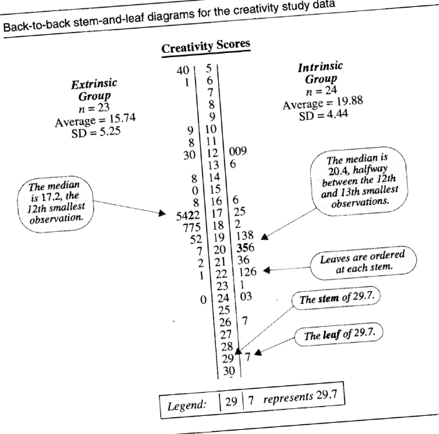
Definition: checks out.
Checklist: yes; true;
P.S
Sorry the picture is tilted, its from a pdf online and that is the best I was able to extract from it.
1.5.4
In (sampling units such as lakes of different sizes)[1], it is sometimes useful to allow (larger units to have higher probabilities of being sampled than smaller units)[2].
Claims: In [1], it is sometimes useful to allow [2].
Subject: While [1], how often [2] is useful.
Predicate: is sometimes useful.
Example: No examples in the chapter.
Definition: -
Checklist: yes; neither;; no-example;
1.5.5
(Close examination of the results of randomization or random sampling)[1] can usually expose ways in which (the chosen sample is not representative)[2]. The (key)[3], however is not to abandon (the procedure when its result is suspect)[4].
Claims: [1] can usually expose ways in which [2].
Subject: What [1], exposes.
Predicate: exposes ways in which [2].
Example: -
Definition: -
Checklist: yes; neither; no-example;
Claims: Not to abandon [4], is key.
Subject: Consequences of not abandoning [4].
Predicate: is key
Example: -
Definition: -
Checklist: yes; neither; no-example;
If (randomization were abandoned)[5], there would be no way to express (uncertainty accurately)[6].
Claims: If [5], there would be no way to express [6].
Subject: If [5], ways to express [6].
Predicate: do not exist
Example: No idea how the example will look
Definition:
Checklist: yes; false; no-example; failed; Pattern: false; no-way-to-do-X
1.6
(Randomized experiments)[1] eliminate (this problem (of confounding variables))[2] by ensuring that differences between groups (other than those of the assigned treatments) are due to chance alone. Statistical measures of uncertainty account for this chance.
Claims: [1] eliminate [2].
Subject: What [1], eliminates.
Predicate: eliminates [2].
Example: I again think that the only way to give an example for these claims is by taking an example and comparing it to reality. That’s how we know we eliminate the problem. For example, I would take the creativity study and then show the effect of confounding variables when randomized and when not randomized. But I don’t have data for this.
Definition: -
Checklist: yes; neither; no-example; failed (because I don’t know how the example is expected to look). Pattern: “Randomized-experiments”; “confounding variables”;
When the model corresponds to the planned use of randomization or random sampling, it provides a firm basis for drawing inferences.
I can know if something provides a firm basis for drawing inferences, only if I get feedback from reality.
Regarding randomization, I have only the creativity study and that is not enough for this claim. I am unable to design the experiment and use R to simulate it. Unable!
Regarding random sampling, the claim is already proven with a simulation in R.
Checklist: yes; neither; no-example; failed (I don’t even know how to simulate such an experiment on randomization)
Chapter 2
2.0 t-distributions
The t-tools are useful in regression and analysis of variance structures
Example out of scope for this chapter
The t-tools are derived under random sampling models when populations are normally distributed.
Subject: What the t-tools are derived under.
Predicate: random sampling models when populations are normally distributed.
Example: I guess I can give an example for t-tools being used when the population is normally distributed and checking if the t-tools give “good” results. Or I could cite the derivation.
Theorem stating: “If Ybar is the average in a random sample of size n from a normally distributed population, the sampling distribution of its t-ratio is described by Student’s t-distribution.”
What should I do?
Definition: -
Checklist: not-sure;neither no-example; failed; (am I even expected to give an example or not.)
2.1.1 Bumpus’s data
As evidence in support of (natural selection)[1], he presented (measurements on house sparrows brought to the Anatomical Laboratory of Brown university after an uncommonly severe winter storm)[2].
Claims: [2] is evidence in support of [1].
Example: Difference in lengths between the armbone of 24 adult male sparrows that perished and 35 adult males that survived. Two sided p-value is 8%.
Definition: A p-value of 8% seems to suggest only a small chance that the null hypothesis is true. This seems to be evidence in support of natural selection, NOT PROOF.
Checklist: yes; true; example-matching-definition; time;
2.1.2 Anatomical Abnormalities Associated with Schizophrenia
Are there any physiological indicators associated with schizophrenia? Yes.
Claims: ^^
Example: Paired difference of hippocampus volume between 15 sets of twins (there by controlling for genes and socioeconomic differences):
- average : 0.199cm^3
- SD : 0.238
- p-value : 0.6%
Definition: This p-value seems to suggest that the null hypothesis (that there is not difference between hippocampus volume of the twins), has a low chance of being true. In other words there seems to be a good chance that there are physiological indicators associated with schizophrenia.
Checklist: yes; true;
2.2.1 One-sample t-tools and paired t-test
The mean of the sampling distribution of the average is also mu, the (standard deviation of the sampling distribution)[1] is (sigma by root n)[2]. The (shape of the sampling distribution)[3] is more nearly normal than is the (shape of the population distribution)[4]. The last fact comes from the Central limit theorem.
Claims: [1] is [2].
Example: Randomly sampled in R was, 10000 numbers from Poisson with lambda=1 (doesn’t look normal at all). And these are the findings:
- n_sample=100
- sd(population)/sqrt(100)=0.10008 [2]
- sd(sampling distribution of the average)=0.1004 [1]
Definition: Checks out!
Checklist: yes; true; ; not-chapter
Claims: [3] is more nearly normal than is [4].
Example: In the above case I took a Poisson distribution with lambda=1; No one in their right mind would say it looks normally distributed.
Contrast that to the sampling distribution of the average and it looks like a bell curve for the example mentioned in the previous claim.
Definition: checks out!
Checklist: yes; true;
The (standard deviation in the sampling distribution of an average)[1], denoted by SD(Y_bar), is the (typical size of (Y_bar-mu))[2], the error in using Y_bar as an estimate of mu. This standard deviation gets smaller as the sample size increases.
Claims: [1] is [2].
Example:
SD(Y_bar) = 0.10008 Ybar-mu = 1.02-1.0045 = 0.0155
Definition: I don’t think it checks out. I suspect I made a mistake with understanding what they meant by “typical size of (Ybar-mu)”. Also if you look at it, Ybar can take any value in the whole sampling distribution depending on chance. So you will never have the same “Ybar-mu”.
Checklist: yes; false; example-matching-subject; failed; Pattern: Y_bar-mu
2.2.3 The T-ratio based on a sample average (start from here)
If the (sampling distribution of the estimate)[1] is normal, then the (sampling distribution of Z)[2] is (standard normal)[3], where the mean is 0 and the standard deviation is 1.
Z = (estimated mean - Mean of population)/SD(estimate)
Claims: If [1] is normal, then [2] is [3].
Example: We go further with the same example we have seen till now
where a population is setup using rpois (Poisson distribution).
[1] looks normal (visually, like a bell curve). Now we compute sampling distribution of Z and determine SD and mean.
mean = 0.009 SD = 1
Definition: Standard normal is defined by SD=1 and mean=0, i.e., checks out.
Checklist: yes; true; if-then
The t-ratio does not have a standard normal distribution, because there is extra variability due to estimating the standard deviation
Subject: What t-ratio matches with.
Predicate: does not match standard normal distribution
Example: We take a Poisson’s distribution with 10000 random
values and lambda=1. pop.mu=0.995 & pop.sd=0.99.
t-ratio = (estimate-parameter)/std.error
In our case, t-ratio = (sample.mn-population.mn)/std.error.
We take 100 samples and 10 units per sample. We compute the tratio and display its mean and sd():
mean : 0.08 sd : 1.16
The mean and sd for Zratio are:
mean: 0.069 sd: 1.00
Definition: For a std normal mean=0; and sd=1; There will always be some error in the values of mean and sd of the sampling distribution. To understand how much error still allows the distribution to be called normal, it seems to be worthwhile to have a look at the Zratio which is expected to be std.normal if the sampling distribution is normally distributed (which is the case here).
Looking at the t-ratio we see that it is not as std-normal as the Z-ratio.
Checklist: yes; true; none; not-chapter; example-matching-subject; time; Pattern: no-idea;
The fewer the (degrees of freedom)[1], the greater is (the extra variability)[2], due to (estimating the standard deviation)[3].
Claims: The fewer the [1], the greater the [2], due to [3].
Checklist: yes; neither. because-should-due-to; almost-missed
Claims: The fewer the [1], the greater is [2].
Example:
With 9 dofs the t-ratio sd: 1.2
with 99 dofs the t-ratio sd: 1.06
Definition: checks out!
Checklist: yes; true; not-chapter;
Under some conditions, however, the sampling distribution of the t-ratio is known.
Claims: Same as below.
if (Y_bar is the average in a random sample of size n from a normally distributed population)[1], (the sampling distribution of its t-ratio)[2] is described by (a student’s t-distribution on n-1 degrees of freedom)[3].
Claims: If [1], [2] is described by [3].
Example: We take a normally distributed population using rnorm
of size 100,000 and compute the t-ratio for a sampling distribution
with sample size 10. We take 10,000 samples and the t-ratios are
computed. We take a population of 10,000 based on rt which samples
from a student’s t-distribution. We compute the mean and sd of the
t-dist with n-1=9 dofs. The mean and sd are tabulated as below:
| zratio | tratio | Students T-distribution | |
|---|---|---|---|
| mean | -0.003 | 0.0012 | 0.005 |
| sd | 1.009 | 1.15 | 1.13 |
Definition: There is a close match between the standard deviations but the match between the means don’t seem to exist. I don’t know why and where the error in the mean is coming from.
Checklist: yes; false; example-matching-definition; failed; (one of us is wrong and it is most likely me.); Pattern: “t-distribution”?; “someone-is-wrong”
Histograms for t-distributions are symmetric about zero. For large degrees of freedom, t-distributions differ very little from the standard normal. For smaller dofs, they have longer rails than normal.
Seem to be simple enough to test with come R-code. Not going to work on it as I am interested in failures.
2.2.4 Unraveling the t-ratio
If the (sample produces one of the 95% most likely t-ratios)[1], then mu is (expected to be) (between 0.067 and 0.331)[2]. <– This is in the case that sample mean is 0.199 and SE is 0.0615 and is part of the Schizophrenia study in Section 2.1.2.
I don’t think I can prove this without the “expected to be”. So I added it. At max I can comment on it based on the t-distribution.
Subject: If [1], what mu is (expected to be).
Predicate: [2]
Example: We come back to the twins study where one of the twins is schizophrenic.
Here the estimate average of differences between the volume is 0.199 cm^3. The SE is determined to be 0.0615.
We know that we are expecting a t-distribution with 14 degrees of freedom. We look at the 2.5th percentile and 97.5th percentile (95% most likely values). The t-ratios are -2.145 and +2.145. This gives us possible values of mu if the sample was drawn with the 95% most likely values.
-2.145<(0.199-mu)/0.615<2.145
This gives 0.067 and 0.331
Definition: Check!
Checklist: yes; true; example-matching-definition; time
(A 95% confidence interval)[1] will contain (the parameter)[2] if (the t-ratio from the observed data happens to be one of the those in the middle 95% of the sampling distribution)[3]. Since 95% of all possible pairs of samples lead to such t-ratios, the procedure of constructing a 95% confidence interval is successful in capturing the parameter of interest in 95% of its applications. It is impossible to say (whether it is successful or not in any particular application)[5].
Claims: if [3], [1] will contain [2].
Subject: if [3], what [1] will contain.
Predicate: will contain [2].
Example: We take a population of mean 0 and sd 1.
For [1] we take a random sample with 100 units where we compute our expected 95% confidence interval for the mean. We compute it as follows:
## compute sample, se and q
x.sam <- x[sample(1:length(x),size=n.sample)]
se <- sd(x.sam)/sqrt(n.sample)
q <- qt(0.975,df=n.sample-1) ## 95% quantiles

## Computing 95%CI
mean(x.sam) + q*se
mean(x.sam) - q*se
-0.011 to 0.34.
For [2] we think of the mean of the population i.e., 0.
For [3], with the below code we get the t-ratio as 1.85. This is
within the middle 95% t-sampling distribution for dof=99, i.e., -1.98
to 1.98.
tratio <- (mean(x.sam)-0)/sd(x.sam)*sqrt(n.sample)
tratio
Definition: We thus see that the CI (-0.011 to 0.34) contains
the mean (the population mean/parameter 0), when the t-ratio is
within the middle 95% of the t-sampling distribution. I checked this
for a couple of random samples and it checked out for all.
took me 3-4 hrs my-god! Seems so simple, but even on the second revision of this post it took me 10mins to make sure I did the right thing. The 3-4 hrs was mainly because I wanted to give an example such that I showed [3] but at the ends of the 95% band. I have still not figured out how to do it.
Checklist: yes; true;;; if; example-matching-definition; time;
Claims: To say [5] is impossible.
No idea how to go about this
Checklist: yes; neither; no-example; failed; Pattern: impossible;
2.3.1 Sampling dist of the diff between 2 independent sample averages
The spread of the sampling distribution will be smaller with larger sample sizes. The sampling distribution is approximately normal, and will be more so with larger sample sizes. As was the case in Section 2.2.1, (the theoretical results about the sampling distribution of Y2-Y1)[1] are insufficient for (making inferential statements)[2], because
SD(Y1_bar-Y2_bar), the standard deviation of this sampling distribution, depends on unknown parameters.
Claims: [1] are insufficient for [2].
Subject: [1] for making [2].
Predicate: are insufficient.
Example: I don’t understand what they mean by [1] or [2] (i.e., I don’t have an example for each)
Definition: -
Checklist: yes; neither; no-example; failed; Pattern: “inferential-statements”; “theoretical results about the sampling distribution”
2.3.2 SE for diff of 2 averages
However, (comparing averages)[1] provides a (complete analysis)[3] only if (all other features of the two distributions are similar)[2]. Therefore assume in the following that the two populations have equal standard deviations: sigma1 = sigma2 = sigma
Subject: If [2], then what [1], provides.
Predicate: provides [3].
Example: No example provided.
Definition: Also definition unclear
Checklist: yes; neither. no-example; failed; definition-unclear (not sure at all what this [3] could be) Pattern: “complete-analysis”
2.3.3 CI for diff between pop means
If the populations are normally distributed, this t-ratio has a t-distribution with n1 + n2 -2 degrees of freedom.
I skip this, as it is simple to test and can be simulated in R.
Now a (statement about the likely values for the t-ratio from the distribution)[1] can be translated into a statement about (the plausible values for mu2-mu1)[2].
Subject: [1] translating to [2].
Predicate: can be translated.
Example: For the Bumpus data of the birds that died vs survived, we look at the Humerus length.
For [1], we think of 95% middle t-ratios from the t-distribution with 57 dofs: 2.002 and -2.002.
For [2], we think computing the possible values of the mean using [1] based on the formula below:
t-ratio = (estimate-mean_under_null_hypothesis)/SE
We have difference in sample mean, i.e., estimate =
(Y2_bar-Y1_bar)=0.01008, along with the SE=0.00567.
We have t-ratio from [1], from which we calculate [2] to be:
-0.00127 < mean_under_null_hypothesis < 0.02143.
Definition: checks out.
Checklist: yes; true;
There is a trade-off between the level of confidence and the width of the confidence interval. The level of confidence can be specified to be large by the user (and a (high confidence level)[1] is (good)[2]). but only at the expense of having (wider interval)[3] (which is (bad)[4] since the interval is less specific in answering the question of interest).
Claims: [1] is good.
Checklist: yes; neither; no-example; failed; (as it is important)
Claims: [3] is bad.
Checklist: yes; neither; no-example; failed; (as it is important)
2.3.4 Testing a hypothesis about diff between means
The p-value may be based on a probability model induced by random assignment in a randomized experiment (section 1.3.2) or on a probability model induced by random sampling from populations, as here.
If the p-value is small, then either the hypothesis is correct—and the sample happened to be one of those rare ones that produce such an unusual t-ratio—or the hypothesis is incorrect. Although it is impossible to know which of these two possibilities is true, the p-value indicates the probability of the first of these results.
Claims: It is impossible to know which of these…
Checklist: yes; neither; no-example ; failed; Pattern: impossible
The smaller the p-value, the stronger is the evidence that the hypothesis is incorrect. A large p-value implies that the study is not capable of excluding the null hypothesis as a possible explanation for how the data turned out. A possible wording in this case is “the data are consistent with the hypothesis being true”. It is wrong to conclude that the null hypothesis is true.
I can take two samples in R and empirically show that the smaller the p-value, the stronger the evidence that the hypothesis is incorrect. I skip this for now.
2.4 Inferences in a two-treatment randomized experiment
Chapter 2 has thus far discussed inference procedures whose motivation stems from considerations of random sampling from populations that are conceptual, infinite, and normally distributed. While there seems to be considerable difference between the situations, it turns out that the (t-distribution uncertainty measures discussed in this chapter)[1] are (useful approximations to both the randomization and the random sampling uncertainty measures for a wide range of problems)[2]. The practical consequence is that t-tools are used for many situations that do not conform to the strict model upon which the t-tools are based, including data from randomized experiments. Conclusions from randomized experiments, however, are phrased in the language of treatment effects and causation, rather than differences in population means and association.
Claims: t-tools are derived under random sampling models, when populations are normally distributed.
Same claim as before in section 2.0.
Checklist: yes; true; no-example; failed; (am I even expected to give an example or not.); Pattern: “derived”;
Claims: [1] for randomization is a useful approximation.
Subject: The usefulness of [1] for randomization
Predicate: is useful approximation
Example: We go back to the creativity study we saw in the first chapter. Here, a group of “creative people” were picked and then randomized into two interventions. The goal is to identify causal relations between the intervention and the creativity score.
In total there were 47 people split as 23 and 24, into the different interventions namely intrinsic and extrinsic.
Using the T-tools for randomization: For the given group we have the
t-statistic = (4.14-0)/1.42 = 2.92. This gives a 0.0027 p-value when
looked up on a t-distribution of 45 dofs.
The above describes “[1] for randomization”.
Using the randomization procedure and a computer simulation with 500 random assignments of the people into the two groups, the real p-value is 0.002.
Definition: The actual p-value and the approximation as a result of [1], seem to be quite close (35% error). All we need for t-tools is a table of values. But to determine actual values you need a computer to perform randomizations. Hence it is a useful approximation.
Checklist: yes; true; example-matching-definition; time;
Claims: [1] for random sampling is a useful approximation.
Just as above was done for randomizations we can establish one for random sampling based on the sex discrimination study; Not done in the book. I skip this for now.
Checklist: yes; true; no-example;
The (randomization-based procedure)[1] (to determine the CI) relies on (a relationship between testing and confidence intervals)[2]: Any hypothesized parameter value should be included or excluded from 100(1-alpha)% confidence interval according to whether its test yields a two-sided p-value that is greater than or less than alpha.
Claims: [1] to determine the CI relies on testing and CI.
Subject: What [1] relies on.
Predicate: relies on testing and CI.
Example: We look at the same creativity study.
The “randomization procedure to determine the CI” ([1]) of creativity study starts with looking at one value of delta.
Let’s say delta=5. We subtract 5 from all scores in the intrinsic group. Now with this homogeneous mixture, we perform the randomization and check if the estimate has a greater probability than the two-sided p-value. If so, then that delta=5 is within the 95% confidence interval.
By trial and error we keep shifting delta’s value to find the limits of this 95% CI.
Definition: This procedure has 2 parts to it. First step involves: Taking each hypothesized parameter value (delta=5) and then TESTING if that probability of delta value is likely (i.e., >5% p-value). The second step involves: doing this until you find the CI limits.
TESTING over and over again seems to lead CI. Claim checks out.
Checklist: yes; true; example-matching-definition; time; Pattern: “CI-testing”; “randomization based procedure”;
Claims: There is a (relationship between testing and confidence intervals)[1].
I don’t have an example for this. I don’t understand how to give example for [1]. CI and Testing are connected as shown above. But that’s all I can tell right now.
This is really hard. How long it takes to understand this is still puzzling. >3hrs easily and no answer. How to show the relationship is unclear in this case.
Checklist: yes; neither; no-example; failed; time; (>3 hrs) Pattern: “relationship”; “testing”; “CI”
2.5 Related issues
Claims: It is difficult and unwise to decide on absolute cutoff points for p-values in all situations.
Subject: How difficult and unwise, absolute cutoff points for p-values is.
Predicate: are difficult and unwise
Example: If we take the absolute cutoff point to be 5%, and we get
a sample with 5.1% p-value then we accept the null hypothesis. If we
get 4.9%, then we are going to reject the null hypothesis.
Although important for leading to advances in the theory of
statistics. The rejection region approach has largely been discarded
for practical applications and p-values are reported instead.
I don’t have an actual example for this.
Definition: Looks like choosing 5% and saying it is valid for
all cases as a hard cut-off seems to be difficult. Also choosing 5%
seems to be unwise as this would result in 2 very close percentages
being interpreted completely differently.
Checklist: yes; true; no-example;
Writing out the subject and predicate is not overrated after all. helps me decide what I need to give an example for.
Claims: p-values can be comprehended by comparing them to events whose probabilities are more familiar.
Subject: Comparing p-values to events whose probabilities are more familiar
Predicate: makes them comprehensible.
Example: We look at the probabilities with respect to a fair
coin.
p(4 heads in a row) = 6.3%
P(5 heads in a row) = 3.1%
P(6 heads in a row) = 1.5%
P(10 heads in a row) = 0.1%
If we get a p-value of 0.1% we think that it is “rare”? Why? Unable to test claim.
I suspect or remember reading somewhere, that p-value cutoffs are intentionally different for different scenarios (unverified claim). Whereas in the above we are comparing one p-value in one scenario to another p-value in say genetics or something.
Definition: I don’t know what “comprehensible” means here or how to check it. Also, I am afraid it is dangerous to compare two p-values from 2 different scenarios.
Checklist: yes; neither; no-example; time; failed; definition-unclear; very very hard; Pattern: “comprehended”; “comparing”; “p-values”
Claims: The actual confidence levels are not important for some cases.
Example: Experiments were made to understand the value of the
parameter “general relativity” (gamma) and to see who was
right. Newton made a 0 prediction and Einstein made a prediction
of 1. A graph showing the value of gamma over several years of
experimentation, shows values ranging from 0.6 to 1.2 in 1920, to 0.95
to 1.05 in 1985. Just this was enough to show that the value of gamma
was closer to one than 0 from 1920 to 1985.
Definition: The whole spread of the gamma values shows that in 1920 the value was close to 1 rather than 0. The CI was not important here but just the whole spread of values was taken.
Checklist: yes; true;
Chapter 3 a closer look at assumptions (2)
3.1.1 Cloud seeding to increase rainfall (1)
(Massive injection of silver iodide into cumulus clouds)[1] can lead to (increased rainfall)[2].
Claims: [1] can lead to [2].
Example: Clouding seeding to increase rainfall randomized experiment:
On 52 days that were deemed suitable for cloud seeding, a random mechanism was used to decide whether to seed the target on that day or to leave it unseeded as a control. An airplane flew in either cases. Precipitation was measured on those 52 days.
Estimate = 3.1 times as large as when not seeded. 95% CI is 1.3 times to 7.7 times.
Definition: Since randomization was used, it is safe to infer causality. Checks out.
Checklist: yes; true;
3.1.2 Effects of Agent Orange on Troops in Vietnam (2)
Dioxin levels tends to be higher for the Vietnam veterans than for the non-Vietnam veterans.
Claims: Dioxin levels in Vietnam Veterans than the non-Vietnam veterans is higher
Example: Agent Orange Study :
In a non-randomly selected sample of 646 Vietnam veterans who served in Vietnam in most heavily treated regions with Agent Orange (Dioxin) were selected as the test group. 97 non-Vietnam veterans who served in US and Germany were the control. Blood tests were done on Dioxin levels reported.
A one-sided p-value of 0.4 for the null hypothesis was obtained.
Definition: The p-value of 40% informs that there is not sufficient evidence to conclude that the levels are higher for the test group than the control.
Caveat: As the sample was not randomly selected, we need to investigate more. For example, non-participating Vietnam veterans may have failed to participate because of dioxin-related illnesses. At best we can say there isn’t sufficient evidence and that the results could be seriously biased.
Checklist: yes; neither;
Inference to populations is speculative.
Not sure how to give an example in this context as there is no data of the true reality to compare with (here). However we have seen before that without randomness inference to population is speculative.
Checklist: yes; neither;
no-example;
3.2.1 The meaning of robustness (2)
Actual conditions did not seem to match the ideal models upon which t-tools are based for both studies.
Claims: The conditions of the Seeded Rainfall study do not match the ideal model on which t-tools are based upon.
Example: When we look at the box plots of the Seeded and Unseeded samples (n=26), we see that the box plots has outliers at 2500 units, when the median is at 250 units and the 75th percentile is at 750 units. There is ~15% of outliers, making it NON-NORMAL (highly skewed).
In addition the SD seen for now as the distance between 25th and 75th percentile in the box plot are ranging from 0 to 750 units in the “Seeded” group and 0 to 450 units in the other group. I.E., different SD’s for different groups.
Definition: Checks out that the normality is not met along with the standard deviations of the populations being not equal (In this case it is only possible to measure the standard deviation of the sample).
Checklist: yes; true.
Claims: The conditions of the Agent Orange study do not match the ideal model on which t-tools are based upon.
Example: We look at the box plot of the Vietnam study. We see again similar trends in outliers as in the last example. The outliers are >4times the 75th percentile. AKA making making it NON-normal.
Looking at the SD or spread, it appears that for both groups the range is same about: 0 to 8 units.
Definition: Checks out! Only the non-normality is not met.
Checklist: yes;true
3.2.2 Robustness Against Departures from normality (6)
Underlying normality is not a serious issue, as long as sample size are reasonably large.
no-example; but it should be possible to simulate in a computer if needed.
Many empirical investigations and related theory, however confirm that the t-tools remain reasonably valid in large samples
no-example (in the book). But can be simulated in a computer if needed.
If the two populations have same (SD and approximately shapes)[1], and if the (sample sizes)[2] are equal, then the (validity of the t-tools)[3] is affected moderately by (long-tailedness)[4] and very little by (skewness)[5].
Claims: If [1] is same, and if [2] is equal, then [3] is affected moderately by [4].
Example: 1000 computer simulations involving a success criterion that 95% of the simulations will contain the parameter of interest were performed. All the populations have the same SD and same sample sizes.
For a given sample size and SD being equal in the population, we see that using t-tools we get the following:
| Sample size | Long tail | Short tail |
|---|---|---|
| 5 | 98.3% | 94.5% |
I suspect that you are going to ask me what Long tail and short tail means. The book has some pictures of how it could look but does not provide actual rules of thumb to identify them.
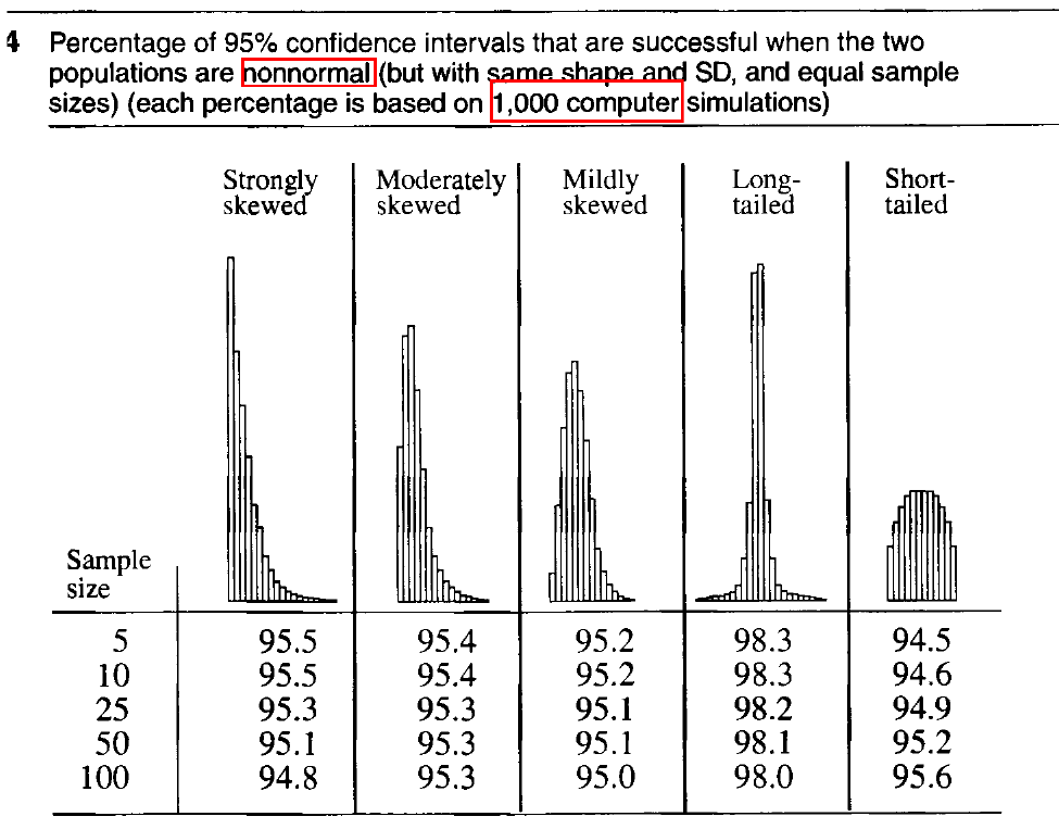
Definition: Looking at the output it looks like the output is good for both short tailed and longtailed non-normal distributions. I am not sure it affects at all, let alone moderately. 94.5% is pretty darn close to 95% (which is the criterion for success).
But the book seems to suggest otherwise: “Only the long-tailed distribution appears to have success rates poor enough to cause potentially misleading statements.”
Checklist: yes; FALSE; example-matching-definition; unsure; (book says otherwise);
Claims: If [1] is same, and if [2] is equal, then [3] is affected very little by [5].
Example: Same example but this time we look at the skewedness.
| Sample size | strongly skewed | mildly skewed |
|---|---|---|
| 5 | 95.5% | 95.2% |
Definition: Looks like it is barely affected as expected in the claim.
Claims: If [1] is same, and if [2] is NOT equal, then [3] is affected moderately by [4].
Example: Example not available for this case.
Definition: -
Checklist: yes; neither; no-example
Claims: If [1] is same, and if [2] is NOT equal, then [3] is affected substantially by [5].
Example: Example not available for this case.
Definition: -
Checklist: yes; neither; no-example
Claims: If [5] between the two populations differs considerably, then the tools can be very misleading with small [2].
Example: no-example
Definition: -
Checklist: yes; false; no-example;
Claims: If [5] differs considerably, then the tools can be misleading with moderate [2].
Example: -
Definition: -
Checklist: yes; false; no-example;
Of the five distributions examined, only the long-tailed distribution appears to have success rates that are poor enough to cause potentially misleading statements—and even those are not too bad.
Example:
| size | strg. skewed | Mod. skewed | mild. skewed | longtailed | shorttailed |
|---|---|---|---|---|---|
| 5 | 95.5% | 95.4% | 95.2% | 98.3% | 94.5% |
Definition: The longtailed distribution appears to have only higher success rates than shorttailed. How is that having poor success rates. No Idea.
Checklist: yes; false; example-matching-definition; unsure; (book says otherwise);
3.2.3 Robustness Against Differing Standard Deviations (3-4)
In this case, the pooled estimate of standard deviation does not estimate any population parameter and the standard error formula which uses the pooled estimate of sd, no longer estimates the sd of the difference between sample averages.
no-example but can be tested using simulations.
(t-tools)[1] remain fairly valid when the (standard deviations are unequal)[2], as long as the (sample sizes are roughly the same)[3].
Claims: If [2] and [3], then [1] remain fairly valid.
Example: A computer simulation involving two populations that have different std.deviations but are normal, turns out as below:
For n1=10 and n2=10, and sigma2/sigma1=1/4 ([2]); success rate as a result of simulation is 95.2%.
Definition: [1] remains fairly valid due to the 95% success rate.
Checklist: yes; true;
(For substantially different sigma’s and different n’s the CI are unreliable)[1] (the worst situation is when the ratio of the sd is much different from one another, and the smaller sized sample is from the population with the larger sd)[2].
Claims: [1].
Example:
A computer simulation involving two populations that have different std.deviations but are normal.
For n1=10 and n2=40, and sigma2/sigma1=1/4; success rate as a result of simulation is 71%.
Definition: unreliable indeed.
Checklist: yes; true;
Claims: [2].
Example: Based on 1000 computer simulations on normal distributions.
| n1 | n2 | sd2/sd1 | sd1/sd2 |
|---|---|---|---|
| 10 | 40 | 71% | 99% |
Definition: checks out!
Checklist: yes; false;
3.2.4.1 Cluster effects and Serial effects (2-3)
Cluster effect occurs sometimes when the data have been collected in sub groups. For example, 50 experimental animals may have been collected from 10 litters.
I don’t know what this effect means or what the impact is.
no-example
The serial effect: The other type of dependence commonly encountered is caused in which measurements are taken over time and observations close together in time tend to be more similar than observations collected at distant time points.
no-example
3.2.4.2 Effects of lack of independence (3)
When the independence assumptions are violated, the standard error of the difference of averages is an inappropriate estimate of the sd of the difference in averages.
can be tested but I don’t know how to simulate dependence/independence; no-example
The t-ratio no longer has a t-distribution, and the t-tools may give misleading results.
no-example
It is unwise to use t-tools directly if cluster of serial effects are suspected.
no-example
Checklist: yes; neither; no-example; failed; (it is important to have examples about independence); Pattern: “independence”; “t-tools”;
3.3.1 Outliers and Resistance (3)
Long-tailed population distributions are not the only explanation for outliers.
Example: Contamination could be another reason for an outlier.
In the Agent Orange study about US veterans and Dioxin, 2 outliers are identified. The sample was about people who were in Vietnam in Orange rich zones. The two outliers in this study were, one of them was not exposed to herbicides during his stay in Vietnam. The other had 180 days of indirect military exposure to herbicides.
Definition: checks out
Checklist: yes; true.
It is irrelevant to distinguish between a natural long-tailed distribution and the one that includes outliers that result from contamination.
no-example The idea is that it becomes irrelevant because they both don’t capture the group behavior. But how would I give an example for that?
Checklist: no; neither;
no-example; failed; Pattern: “irrelevant”
It is useful to know how sensitive a statistical procedure may be to one or two outlying observations.
Example: We comeback to the same Agent Orange data. We have two outliers here. The sample size is >600 in the case of veterans in Vietnam.
The one-sided p-value is 40% with all observations, 48% with one outlier removed and 54% with both outliers removed.
Definition: Although the conclusion didn’t change regarding rejecting or accepting an hypothesis, the variation is quite large between keeping outliers despite the large number of the sample.
This example I think checks out that it is useful. I think this example is instrumental in showing the havoc, outliers can breathe when values become closer to the “cutoff”(say 5%)
Checklist: yes; true;
3.3.2 Resistance of t-tools (2)
Since t-tools are based on averages, they are not resistant
Claims: t-tools are not resistant to outliers
Example: In a hypothetical sample of 10,20,30,50,70, the sample
average is 36, and the sample median is 30. Now change the 70 to 700,
and we see that the average becomes 162, but the sample median remains
30.
no-example; Can be simulated.
Definition: -
Checklist: yes; true; no-example;
one or two outliers can affect the CI or change the p-value enough to completely alter a conclusion.
no-example
3.4.1 Consider Serial cluster effects (1)
Were the subjects selected in distinct groups? Were different Groups of subjects treated differently in a way that was unrelated to the primary treatment? Were different responses merely repeated measurements of the same subjects? Were observations taken at different but proximate times or locations? Affirmative answers to any of these questions suggest that independence may be lacking.
Claims: If the answer to above questions is yes then it suggests that independence may be lacking.
Checklist: yes; neither; no-example; definition-unclear; failed (should know how to check for independence but not given in the text clearly); Pattern: “independence”;
3.4.2 Evaluate the suitability of the t-tools (1)
A (transformation)[2] should be considered if the (graphical displays of the transformed data appear to be closer to the ideal conditions)[1].
Subject: If [1], Should [2] be done?
Predicate: should be considered.
Example: We go back to the Cloud seeding case study. We see in the normal box plots that both the groups look “skewed”. And the spread (SD) looks much larger for the seeded one.
When we make this into a logarithm chart we see that immediately the spreads look very similar (SD similar), the skewness vanishes (closer to normal looking). These are conditions that are close to what the t-tools are created based on.
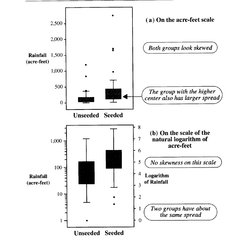
Definition: Checks out. We should consider it as the transformation could make your data look more applicable to the t-tools.
Something more nicer would be to check the results of using the actual values and the transformed values and seeing how different the results are.
Checklist: yes; true;
3.4.3 A strategy for Dealing with Outliers (2)
If investigation reveals that an outlying observation was recorded improperly or was the result of contamination from another population, the solution is to correct it if the right value is known or to leave it out.
Example: We comeback to the same Agent Orange study. We have two outliers here. The sample size is >600 in the case of veterans in Vietnam.
The one-sided p-value is 40% with all observations, 48% with one outlier removed and 54% with both outliers removed.
Here even though it does not affect the conclusion of this study, the variation in the p-value is 14%.
Definition: Quite a large variation, and by removing them we are more closer to the truth (without contaminants).
This is the best example I have, unfortunately it doesn’t show a failing case.
Checklist: yes; neither;
An important aspect of adopting this procedure is that an outlier does not get swept under the rug simply
because it is different from the other observations.
Claims: Using careful examination as shown in fig.3.7, we prevent contaminants from influencing the result.
Subject: Prevention of using careful examination
Predicate: prevent contaminants from influencing the result.
Example: We take the same example as before. We find the contaminants and remove them there by not allowing the contaminants to affect the result.
Definition: Checks out.
Checklist: yes;true; subject-predicate-split; unsure; time; (15 mins); “Using XYZ, we do ABC”
3.4.4 Agent orange (2)
the skewness is mild and unlikely to cause any problems with the t-test or the CI (for the Agent orange study)
Claims: The skewness in Agent Orange study is mild
Example: We look at the skewness below (pg67). Here the tail is long on one side and there seems to be a relatively smaller tail on the other side.
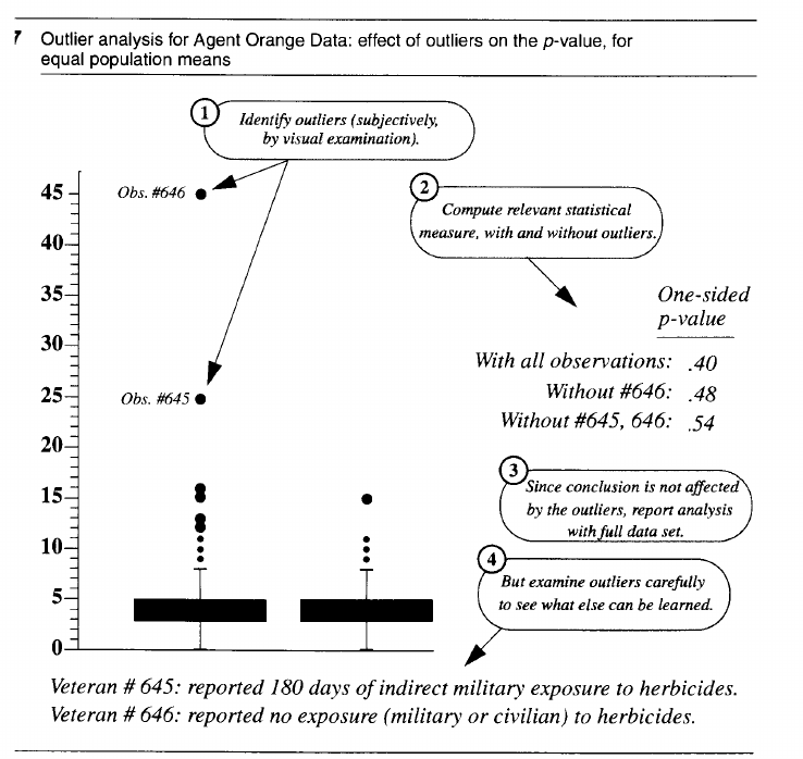
Definition: Looking at the picture below (pg61) describing mild skewness, we see that a mild skewness looks such that there are tails on both sides, but the tail on one side is shorter.
Yes it seems quite subjective, as the book does not seem to want to quantify it
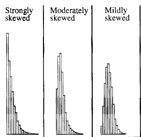
Checklist: yes; true.
Claims: The skewness is unlikely to cause any problems with t-test or the CI.
Example: It is possible to run a computer simulation on a similar problem based on this skewness and number of units in a sample, to test it. But not for this exact study.
Definition: -
Checklist: yes; neither no-example
3.5.1 The Logarithmic Transformation (1)
The most useful transformation is the logarithm for positive data.
It is unclear against what dimensions this is most useful. I could probably show in an example, say with the Vietnam war study, that log works better in this case, but going to MOST from here I have no idea how to go about it.
Checklist: yes; neither; most; no-example ;failed; Pattern: most; “lack-of-examples”
3.5.1.1 Recognizing the need for Log (5)
The data themselves usually suggest the need for a log transformation. If the ratio of the largest to the smallest measurement in a group is greater than 10, then the data are probably more conveniently expressed on the log scale. If the (graphical displays of the two samples show them both to be skewed)[1] and if (the group with the larger average also has the larger spread)[2], the (log transformation)[3] is likely to be a good choice.
Claims: If [1] and [2], then [3] is a good choice.
Example: We take the cloud seeding example. We plot the box plot and see that the data is “moderately skewed” (according to some graphical display on pg61). Also the seeded group has much larger spread (median @250 and extreme at 2500), than unseeded (median @150 and extreme at 1250).
Taking log transforms we get two groups that have the same spread and very little skewness.
Definition: The initial groups aren’t expected to work with t-tools due to long-tailedness of the sample (as seen before). After transformation they would work with t-tools as there is no skewness or long-tailedness and both groups have the same spread, which is what the t-tools can work reliably on (as seen before).
Checklist: yes; true; example-matching-definition; time (20mins).
The overall result is that the (two distributions on the transformed scale)[1] appear to be (symmetric and have equal spread)[2]— just the right conditions for applying the t-tools.
Claims: [1] appears to be [2].
Example: Same example as above.
Definition: checks out.
Checklist: yes; true
Claims: If two distributions have symmetric and equal spread, then they have right conditions for applying t-tools.
Example: Don’t have an example. A computer simulation providing the success rate would be the check.
Definition: -
Checklist: yes; neither; no-example
Small numbers get spread out more, while large numbers are squeezed more closely together (as a result of log transformation)
Example: If you look at a log plot and divide it equally… then this is what you see…
1-10 say corresponds to 2units. 10 to 100 has the same 2 units. And 100 to 1000 has the same 2 units. It can be visualized in the previous figure.
Definition: checks out!
Checklist: yes; true
3.5.2 Interpretation after a Log Transformation (1)
For some measurements, the results of an analysis are appropriately presented on the transformed scale.
Example: The Richter scale is used to measure earthquakes’ strength.
Definition: checks out.
Checklist: yes; true;
3.5.2.2 Population model (5)
Taking the (antilogarithm of the estimate of the mean on the log scale)[1] does not give (an estimate of the mean on the original scale)[2].
Example: For [1] : we get 169.01 for the seeded case in the cloud seeding example.
exp(mean(df$lograin[df$Treatment=="Seeded"]))
For [2], we compute the mean of the rainfall in the original scale = 441
mean(df$Rainfall[df$Treatment=="Seeded"])
Definition: Checks out!
Checklist: yes; true; definition-unclear; time (20mins); Pattern: “long phrases?”
If, log-transformed data have symmetric distributions, then Mean[logY] = Median[logY]
Example:
summary(df$lograin[df$Treatment=="Seeded"])
Min. 1st Qu.  Median    Mean 3rd Qu.    Max.
1.411   4.581   5.396   5.134   6.001   7.918
Definition: Although this treatment does not result in totally symmetric distribution (still has a small tail on one side), it still manages to keep the median and mean close by. So good enough and checks out.
Checklist: yes; true;
It is evident that (the anti logarithm of the mean of the log values)[1] is the (median on the original scale of measurements)[2].
Example: We think of the same cloud seeding example:
For [1] we think of
exp(mean(df$lograin[df$Treatment=="Unseeded"]))
= 54
For [2] we think of
median(df$Rainfall[df$Treatment=="Unseeded"])
= 44
Definition:
summary(df$Rainfall[df$Treatment=="Unseeded"])
Min. 1st Qu.  Median    Mean 3rd Qu.    Max.
1.00   24.82   44.20  164.59  159.20 1202.60
The data taken is not fully symmetric. It still has some tails. Despite that [1] is a close match to the median in the normal scale.
Checklist: yes;true;
A problem with interpretation on the original scale arises
Claims: (A problem)[0] with (interpretation on the original scale)[2] arises if we use (log transformation)[1].
Subject: If [1], Is [2] expected to arise?
Predicate: yes.
Example:
In the case of log transformation (as shown in the previous example):
For [2], we think of the previous example where the ‘antilog of mean of log values’ is the median in the original scale and NOT THE MEAN.
#antilog of mean of log
exp(mean(df$lograin[df$Treatment=="Unseeded"]))
= 54

#Actual mean and median
summary(df$Rainfall[df$Treatment=="Unseeded"])
Min. 1st Qu.  Median    Mean 3rd Qu.    Max.
1.00   24.82   44.20  164.59  159.20 1202.60
Definition: Whether it is a problem I am not sure. I think the author just wanted to inform that you wont get the MEAN anymore in the original scale, after the log transformation—which is true. So I say it checks out.
Checklist: yes; true; example-matching-subject; time; Pattern: “interpretation”; “original-scale”
exp(Z2bar-Z1bar)estimatesMedian(Y2)/Median(Y1)
Claims: ^^
Example: Either I can simulate and show this using computer simulations in R. OR I provide the proof as in the text book. Proof is not an example. So the best I can do is a Computer simulation. I skip these type of simulations now
Definition: -
Checklist: yes; neither; no-example;
The point of the above is that a very useful multiplicative interpretation emerges in terms of the ratio of population medians.
Claims: (Multiplicative interpretation in terms of the ratio of population medians)[1], emerges from the (previous claim)[2].
Question: Does [1] emerge from [2].
Example: So basically there is a log A - log B which becomes
log[A/B]. When you take the antilog you get ratio of A and B. I am
not sure I can show this in an example. I don’t have an example.
Definition: -
Checklist: yes; neither; no-example; failed; time; example-matching-subject; failed; Pattern: “A-emerges-from-B”; “related-to-derivation” (Very hard this was)
Claims: The emerged multiplicative interpretation is very useful.
Example: After using the log transformation and performing the t-test on the Cloud seeding data, we see that the confidence interval suggests that the rainfall is 1.27 times to 7.74 times higher in the case of seeded.
Definition: The log transformation seems to allow to interpret the original data in terms of ratio which is useful to understand the outcome. Not sure how it is “very useful”
Checklist: yes; neither; definition-unclear;
In addition, (back-transforming the ends of a confidence interval constructed on the log scale)[1] produces a (confidence interval for the ratio of medians)[2]
Example: No example.
The only way to show this seems to be through a computer simulation. With the studies given in the book, it is not possible to tally this claim. For example, with the Cloud seeded study, I can compute the confidence intervals on the log scale and back transform it. To check if the number produces a CI of the ratio of medians I have nothing to check it against.
Definition: -
Checklist: yes; neither; no-example;
3.5.2.3 Example (sex discrimination) (1)
Graphical displays of the log-transformed salaries indicate that analysis would also be suitable on the log scale.
Example: Looking at the male and female histograms
hist(df$logSalary[df$Sex=="Male"])
Looks symmetric with very short tail (very little skewness and short-tailed histogram). The spread ranges from 8.4 to 9.0 = 0.6
hist(df$logSalary[df$Sex=="Female"])
Has a small tail (mildly skewed and short-tailed histogram). The spread ranges from 8.26 to 8.74 =0.48
Definition: Both histograms seem to be close to normal and have similar spread which are roughly ideal conditions for applying t-tools, and hence make analysis also suitable for the log scale.
Checklist: yes; true.
3.5.3 Other transformations for Positive measurements (5)
There are other useful transformations for positive measurements with skewed distributions where the means and standard deviations differ between groups.
no-example No example of actually applying another transformation is given.
The square root transformation applies to data that are counts.
no-example
The reciprocal transformation 1/Y applies to data that are waiting time
no-example
The arcsine square root transformation and the logit transformation apply when the measurements are proportions between zero and one.
no-example
Only log gives such ease in converting inferences back to the original scale of measurement.
no-example
Situations arise where presenting results in terms of population medians is not sufficient.
no-example
3.6.1 Prefer Graphical Methods over Formal Tests for Model Adequacy
Tests for normality and tests for equal sd are available in most computer programs.
no-example
The diagnostic tests are not very helpful for model checking.
no-example
Graphical displays provide a good indication of whether or not the data are amenable to t-analysis and, if not, they often suggest a remedy.
Subject: What Graphical displays provide
Predicate: a good indication of … t-analysis
Claim dealt with before with the seeded cloud study in section … ???
Claims: Graphical displays, when data are not amenable to t-analysis, often suggest a remedy.
no-example
3.6.2 Robustness and Transformation for Paired t-Tools (2)
When the (observations within each pair are positive)[1], either (an apparent multiplicative treatment effect (in an experiment))[2] or a tendency for larger differences in pairs with larger average values suggest the use of log transformation.
Dealt with similar claim in section 3.5.1.1
Summary (1)
This is the situation where log-transformation confirms the adequacy of the transformation.
claim discussed before in section 3.5.1.1
General statistics
Over the past 2 months I have been working on this and the essay on “working on failures”. It took a “lot of time” to read and work out the claims, identifying my failures, to find a way to make the first practice session, write some bash scripts etc… Also the books I took were a lot of work (10 claims per hour was very very rare). I can’t remember spending 2 months for roughly 250 claims. In between I also spent time to write some bash scripts that would process my failures and give me stats such as below:
Total claim: 136
Failed: 49 claims
Failure types as seen below:
example-matching-definition: 11
no-example: 23
definition-unclear: 2
subject-predicate-split: 1
example-matching-subject: 8
because-should-due-to: 2
I guess the plan would be to take types where I have failed the most and practice them and follow it up with feedback if it has helped. How do we know if something has helped is to see a SCORE. So for example, if I see only 5 no-example failures instead of 23, in the next practice session of the same books then it would be considered an improvement in Score.
Over the last two months
Amount of effort (not just DPing) put on average per week (not only DPing): 20hrs per week or 2.8 hrs per day avg (Courtesy:Org-mode, PNN). Its not great, its not what I set out for in march which was 4 hrs.
Appendix: Round 1
I try to count distractions (acronym:dist), and how much time I spend per phrase/claim, how much time I spend on reading etc…
Superintelligence
| chapter | time | phrases | dist | claims | pages | mins/phr | mins/pg |
|---|---|---|---|---|---|---|---|
| 2.2 | 10 | 2 | 1 | 1 | (6) | 5 | |
| 2.3 | 60 | 5 | 8 | 7.5 | |||
| 2.3 | 21 | 2 | 0 | (8) | 10 | ||
| 2.4 | 20 | 1 | 4 | 6.25 | |||
| 2.5 | 15 | 1 | 3 | 5 | |||
| 2.4 2.5 | 20 | 2 | 4 | ||||
| 3 | 27 | 5 | 5.4 | ||||
| 3 | 60 | 13 | 6 | 10 | |||
| 3 | 159 | 34 | 9 | 4.67 |
Statistical sleuth
| chapter | time | phrases | dist | claims | pages | mins/phr | mins/pg | date |
|---|---|---|---|---|---|---|---|---|
| 1.1.1 | 19 | 3 | 6.3 | |||||
| 1.1.1 | 40 | 2 | 1 | 20 | ||||
| 1.1.2 | 7 | 2 | 3.5 | |||||
| 1.1.2 | 22 | 2 | 1 | 11.5 | ||||
| 1.2.1,.2 | 60 | 2 | 4 | 15 | ||||
| 1.2.1,2 | 90 | 16 | 8 | 8 | 5.6 | |||
| ” | 60 | 3 | 2 | 2 | 20 | |||
| ”” | 25 | 6 | 1 | 3 | 4.16 | |||
| 1.3.1,2 | 40 | 8 | 4.5 | 8.8 | ||||
| 1.4 | 24 | 4 | 2 | 12 | 3/09 | |||
| 1.5.1 | 48 | 9 | 5 | 9.6 | 3/09 | |||
| 1.2.3 | 90 | 8 | 10 | 4 | 11.25 | 3/09 | ||
| 1.2.3 | 80 | 6 | 9 | 3 | 13.3 | 4/09 | ||
| 1.3.1,2 | 90 | 9 | 11 | 4 | 10 | 4/09 | ||
| 1.4,1.5 | 80 | 9 | 11 | 4 (3) | 8.88 | 4/09 | ||
| 1.5 | 75 | 12 | 15 | 6 | 6.25 | 5/09 | ||
| 2.1,2* | 46 | 7 | 6.57 | 7/09 | ||||
| 2.1 | 45 | 4 | 7 | 2 | 11.25 | 7/09 | ||
| 2.2 | 90 | 8 | 8 | 4 | 7/09 | |||
| 2.2.4,2.3 | 54 | 8 | 6.75 | 8/09 | ||||
| ^^ | 27 | 3 | 9 | 8/09 | ||||
| ^^ | 30 | 4 | 8/09 | |||||
| ^^ | 90 | 3 | 1 | 8/09 | ||||
| ^^ | 100 | 4 | 7 | 2 | 25 | 9/09 | ||
| ^^ | 28 | 2 | 2 | 1 | 9/09 | |||
| ^^ | 80 | 0 | 9 | 0 | 9/09 | |||
| ^^ | 120 | 2 | 8 | 1 | 75 | 10/09 | ||
| ^^ | 45 | 3 | 1 | 15 | 11/09 | |||
| ^^ | 60 | 4 | 9 | 2 | 15 | 11/09 | ||
| 3.1,3.2 | 50 | 9 | 7 | 7.14 | 12/09 | |||
| 33 | 4.5 | 6.66 | 12/09 | |||||
| 60 | 9 | 5 | 12 | 14/09 | ||||
| 13 | 3 | 2.75 | 4.7 | 14/09 | ||||
| 97 | 18 | 8 | 9 | 5.38 | 15/09 | |||
| pr** | 52 | 20 | 2 | 10 | 2.6 | 15/09 | ||
| 35 | 10 | 2 | 5 | 3.5 | 15/09 | |||
| 62 | 18 | 7 | 9 | 3.4 | 16/09 | |||
| 62*** | 10 | 6 | 5 | 6.2 | 16/09 | |||
| 66 | 14 | 7 | 7 | 4.17 | 16/09 | |||
| 18 | 6 | 6 | 3 | 3 | 16/09 | |||
*2 pages of images ** started skipping claims if I had no example, and if I could give a simulation to prove it.
*** took some time due to puzzling as well as using R to setup and make shit happen Pnn!
Corrections
| date | time | Claims | phrases | dist | min/phr | mins/dist | words/min |
|---|---|---|---|---|---|---|---|
| 17/09 | 44 | 2 | 4 | 4 | 11 | 11 | |
| 17/09 | |||||||
| 18/09 | 60 | 10 | 7 | 3 | 8.5 | ||
| 18/09 | 72 | 4 | 8 | 6 | 9 | 12 | |
| 18/09 | 60 | 4 | 8 | 4 | 7.5 | 15 | |
| 19/09 | 54 | 4 | 8 | 7 | 6.75 | 7.7 | |
| 19/09 | 56 | 14 | 28 | 9 | 2 | 6.2 | |
| 19/09 | 53 | 9 | 18 | 8 | 2.94 | 6.6 | |
| 21/09 | 60 | 10 | 20 | 10 | 3 | 6 | |
| 21/09 | 90 | 8 | 16 | 12 | 5.6 | 7.5 | |
| 21/09 | 63 | 15 | 30 | 12 | 2.1 | 5.25 | |
| 21/09 | 28 | 7 | 14 | 8 | 2 | 3.5 | |
| 21/09 | 62 | 9 | 18 | 10 | 3.4 | 6.2 | |
| 22/09 | 30 | 1 | 2 | 3 | 15 | 10 | |
| 22/09 | 30 | 5 | 10 | 4 | 3 | 7.5 | |
| 23/09 | 60 | 10 | 20 | 15 | 3 | 4 | |
| 23/09 | 45 | 10 | 20 | 7 | 2.25 | 6.42 |